11. Functional Programming
The main difference between the functional programming paradigm and other paradigms is that functional programming uses functions rather than statements to express ideas. This difference means that instead of writing a precise set of steps to solve a problem (think like a recipe for building a cake), you use pre-, or user-defined functions, and don’t worry about how the language performs the task. In imperative programming, another example of a programming paradigm, data moves through a series of steps in a specific order to produce a particular result.
This may sound esoteric, but let us consider the simplest example from Excel, with which most people are familiar, where you have been using functional programming all along without realising it! Suppose you had a collection of twenty data points in cells A1:A20 and wanted to calculate the sum of these numbers.
- With imperative programming, you would write a
forloop, declare thatsum = 0, take the next value, add it to the value ofsumand keep track of the running sum, until you have looped all of the values, in whcih case you would just print out the value ofsum. You can actualyl write such a loop, even in Excel, but I don’t think anyone has even bothered - With functional programming, you would use Excel’s built in
=SUM()function and apply the function to the cells that contain your data; namely=SUM(A1:A20).
This idea of applying a function into an array (or vector) is something that is really useful in R. A function can be an Excel-like function of sum, median, etc., but far more importantly R allows us to apply the same thing, say a linear regression model (lm in R talk) into an entire dataframe.
11.1 The map() function
You frequently need to iterate over vectors or data frames, perform an operation on each element, and save the results somewhere. for loops may at first seem more intuitive to use because you are explicitly identifying each component and step of the process. However, you have to track the value over which you are iterating, you need to explicitly create a vector to store the output, you have to assign the output of each iteration to the appropriate element in the output vector, etc.
The purrr package and its map functions allow us to concentrate on the operation being performed (e.g. mean(), median(), max()), not all the extra code needed to make the operation work. The map family of functions mirrors for loops, as they:
- Loop over a vector
- Do something to each element
- Save the results
The arguments of map( .x, .f, ...) are
.xcan be a vector, a list, or a tidy dataframe, as we can apply something to each column. In general, we want to operate on each value/element of.x.f. specifies what to do with each piece. It can be, among others, either- A function, like
mean(). - A formula, which is converted to an anonymous function, so that ~ lm(lifeExp ~ year, data = .) is shorthand for function(x) lm(lifeExp ~ year, data = x).
- A function, like
Map functions come in a few variants based on their inputs and output:
map()returns a list.map_lgl()returns a vector of logical values (TRUE/FALSE).map_int()returns a vector of integersint.map_dbl()returns a vector of real numbersdbl.map_chr()returns a vector of characterschr.
As an example, let us define a dataframe df that contains three variables/columns with 100 random numbers drawn from a Normal distribution with a mean of 0 and standard deviation of 1.
Like all functions in the tidyverse, the first argument is the data object, and the second argument is the function to be applied. Additional arguments for the function to be applied can be specified like this:
# take the tidy dataframe df, and apply the function 'mean' to each element (column), and remove NAs
map_dbl(df, mean, na.rm = TRUE)
## a b c
## 0.01524 0.15587 -0.00328# take the tidy dataframe df, and apply the function 'median' to each element (column), and remove NAs
map_dbl(df, median)## a b c
## -0.0837 0.1639 0.0343# take the tidy dataframe df, and apply the function 'sd' to each element (column), and remove NAs
map_dbl(df, sd)## a b c
## 0.930 0.951 0.884Or we can use the pipe operator %>%, starting with the dataframe and then applying the map_dbl function to it
##        a        b        c
## 0.01524 0.15587 -0.0032811.1.0.1 Mean of numeric columns in gapminder
Let us use a map() function that calculates the arithmetic mean for every numeric column in gapminder. Given that the dataset also has years, countries and continents, we first select the numeric columns of interest, and then apply the mean function
gapminder %>%
  # select only numeric variables/columns
  select(lifeExp, pop, gdpPercap) %>%

  #apply the mean function
  map_dbl(mean,  na.rm = TRUE)
## lifeExp pop gdpPercap
## 5.95e+01 2.96e+07 7.22e+0311.2 Running many regressions
Suppose we wanted to study how life expectancy increased over time on the gapminder dataset. We can plot the relationship for every single country as shown below:
ggplot(gapminder, aes(x=year, y=lifeExp, group=country))+
geom_line(aes(colour=continent))+
  labs(x = "Year", y = "Life expectancy", title = "Life Expectancy improvement 1952-2007") +
  theme_bw()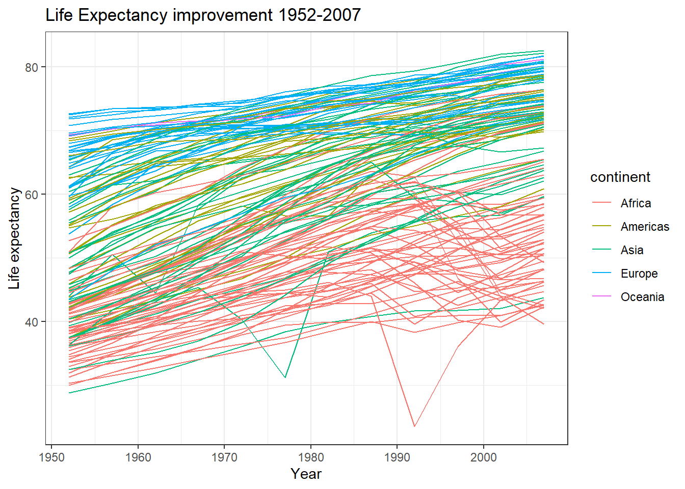
Most of these look like linear relationships and we would like to know the intercept, namely life expectancy in 1952, the first year we have data for, and slope, or the average improvement of life expectancy for each additional year. Let us run a simple regression for one country:
options(digits = 3)
yearMin <- 1952

tempCountry <- "Greece"  # Just a random example
tempData <- gapminder %>%
  filter(country== tempCountry)

tempData
## # A tibble: 12 x 6
## country continent year lifeExp pop gdpPercap
## <fct> <fct> <int> <dbl> <int> <dbl>
## 1 Greece Europe 1952 65.9 7733250 3531.
## 2 Greece Europe 1957 67.9 8096218 4916.
## 3 Greece Europe 1962 69.5 8448233 6017.
## 4 Greece Europe 1967 71 8716441 8513.
## 5 Greece Europe 1972 72.3 8888628 12725.
## 6 Greece Europe 1977 73.7 9308479 14196.
## 7 Greece Europe 1982 75.2 9786480 15268.
## 8 Greece Europe 1987 76.7 9974490 16121.
## 9 Greece Europe 1992 77.0 10325429 17541.
## 10 Greece Europe 1997 77.9 10502372 18748.
## 11 Greece Europe 2002 78.3 10603863 22514.
## 12 Greece Europe 2007 79.5 10706290 27538.ggplot(tempData, aes(x=year, y=lifeExp))+
geom_point() +
geom_smooth(method='lm', se=FALSE)+
labs(x = "Year", y = "Life expectancy", title = "Greece: Life Expectancy improvement 1952-2007") +
theme_bw()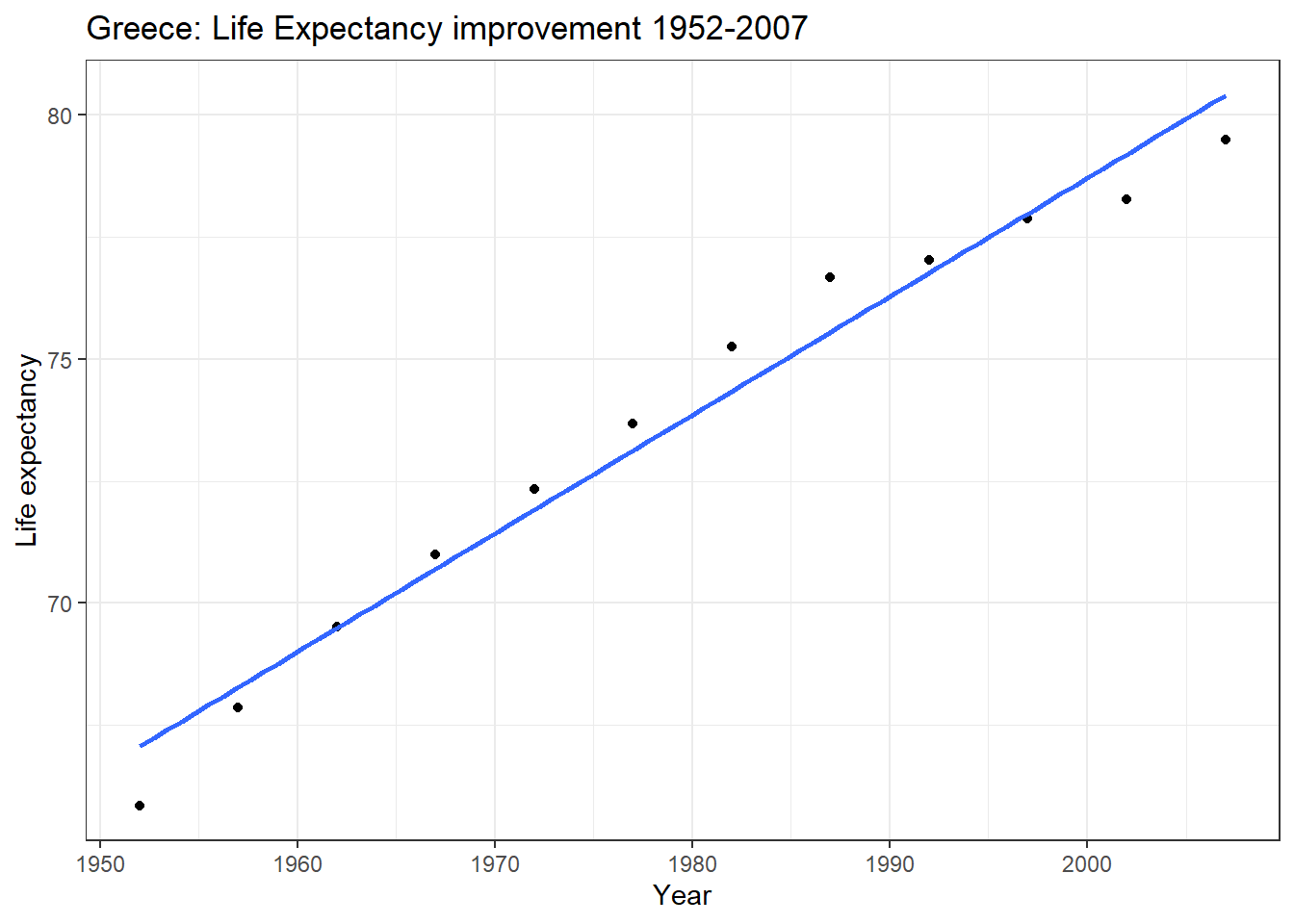
model1 <- lm(lifeExp ~ I(year - yearMin), data=tempData) #fit a linear regression model, lm
coef(model1) #show the coefficients of the regression model, namely the intercept and the slope
## (Intercept) I(year - yearMin)
## 67.067 0.242The intercept of 67 is what our model predicts life expectancy was in 1952– the actual value was 65.9. The slope of 0.242 means that every year between 1952 and 2007, life expectancy increased on average by 0.242 years.
Now, what if we wanted to manipulate the entire gapminder dataframe and running 100s of regressions at once? This is where purrr and map become really useful.
First, we use group_by and nest to create a dataframe that contains dataframes for each country, and then use map to run a regression for each country. Finally, we get the coefficients and all the regression details.
library(broom)
library(forcats)
many_models <- gapminder %>%
  # create a dataframe containing a separate dataframe for each country
  group_by(country,continent) %>%
  nest()  %>%

  # Run a simple regression model for every country in the dataframe
  mutate(simple_model = data %>%
           map(~lm(lifeExp ~ I(year - yearMin), data = .))) %>%

  # extract coefficients and model details with broom::tidy
  mutate(coefs = simple_model %>% map(~ tidy(., conf.int = TRUE)),
         details = simple_model %>% map(glance)) %>%
  ungroup()

head(many_models, 10)
## # A tibble: 10 x 6
## country continent data simple_model coefs details
## <fct> <fct> <list> <list> <list> <list>
## 1 Afghanistan Asia <tibble [12 x 4]> <lm> <tibble [2 x 7]> <tibble [1 x 11]>
## 2 Albania Europe <tibble [12 x 4]> <lm> <tibble [2 x 7]> <tibble [1 x 11]>
## 3 Algeria Africa <tibble [12 x 4]> <lm> <tibble [2 x 7]> <tibble [1 x 11]>
## 4 Angola Africa <tibble [12 x 4]> <lm> <tibble [2 x 7]> <tibble [1 x 11]>
## 5 Argentina Americas <tibble [12 x 4]> <lm> <tibble [2 x 7]> <tibble [1 x 11]>
## 6 Australia Oceania <tibble [12 x 4]> <lm> <tibble [2 x 7]> <tibble [1 x 11]>
## 7 Austria Europe <tibble [12 x 4]> <lm> <tibble [2 x 7]> <tibble [1 x 11]>
## 8 Bahrain Asia <tibble [12 x 4]> <lm> <tibble [2 x 7]> <tibble [1 x 11]>
## 9 Bangladesh Asia <tibble [12 x 4]> <lm> <tibble [2 x 7]> <tibble [1 x 11]>
## 10 Belgium Europe <tibble [12 x 4]> <lm> <tibble [2 x 7]> <tibble [1 x 11]>The resulting dataframe many_models contains for every country the country data, the regression model simple_model, the model coefficients coefs, as well as all the regression details. As discussed earlier, the intercept is the predicted life expectancy in 1952 and the slope is the average yearly improvement in life expectancy.
We will take our many_models dataframe, unnest the coefs and extract the interecept and slope for each country.
intercepts <-
  many_models %>%
  unnest(coefs) %>%
  filter(term == "(Intercept)") %>%
  arrange(estimate) %>%
  mutate(country = fct_inorder(country)) %>%
  select(country, continent, estimate, std.error, conf.low, conf.high)

# let us look at the first 20 intercepts, or life expectancy in 1952
head(intercepts,20)
## # A tibble: 20 x 6
## country continent estimate std.error conf.low conf.high
## <fct> <fct> <dbl> <dbl> <dbl> <dbl>
## 1 Gambia Africa 28.4 0.623 27.0 29.8
## 2 Afghanistan Asia 29.9 0.664 28.4 31.4
## 3 Yemen, Rep. Asia 30.1 0.861 28.2 32.0
## 4 Sierra Leone Africa 30.9 0.448 29.9 31.9
## 5 Guinea Africa 31.6 0.649 30.1 33.0
## 6 Guinea-Bissau Africa 31.7 0.349 31.0 32.5
## 7 Angola Africa 32.1 0.764 30.4 33.8
## 8 Mali Africa 33.1 0.262 32.5 33.6
## 9 Mozambique Africa 34.2 1.24 31.4 37.0
## 10 Equatorial Guinea Africa 34.4 0.178 34.0 34.8
## 11 Nepal Asia 34.4 0.502 33.3 35.5
## 12 Somalia Africa 34.7 1.01 32.4 36.9
## 13 Burkina Faso Africa 34.7 1.11 32.2 37.2
## 14 Niger Africa 35.2 1.19 32.5 37.8
## 15 Eritrea Africa 35.7 0.813 33.9 37.5
## 16 Ethiopia Africa 36.0 0.569 34.8 37.3
## 17 Bangladesh Asia 36.1 0.530 35.0 37.3
## 18 Djibouti Africa 36.3 0.612 34.9 37.6
## 19 Madagascar Africa 36.7 0.304 36.0 37.3
## 20 Senegal Africa 36.7 0.506 35.6 37.9slopes <- many_models %>%
unnest(coefs) %>%
filter(term == "I(year - yearMin)") %>%
arrange(estimate) %>%
mutate(country = fct_inorder(country)) %>%
select(country, continent, estimate, std.error, conf.low, conf.high)
# let us look at the first 20 slopes, or average improvement in life exepctancy per year
head(slopes,20)## # A tibble: 20 x 6
## country continent estimate std.error conf.low conf.high
## <fct> <fct> <dbl> <dbl> <dbl> <dbl>
## 1 Zimbabwe Africa -0.0930 0.121 -0.362 0.175
## 2 Zambia Africa -0.0604 0.0757 -0.229 0.108
## 3 Rwanda Africa -0.0458 0.110 -0.290 0.199
## 4 Botswana Africa 0.0607 0.102 -0.167 0.288
## 5 Congo, Dem. Rep. Africa 0.0939 0.0406 0.00338 0.184
## 6 Swaziland Africa 0.0951 0.111 -0.153 0.343
## 7 Lesotho Africa 0.0956 0.0992 -0.126 0.317
## 8 Liberia Africa 0.0960 0.0297 0.0299 0.162
## 9 Denmark Europe 0.121 0.00667 0.106 0.136
## 10 Uganda Africa 0.122 0.0533 0.00280 0.240
## 11 Hungary Europe 0.124 0.0199 0.0794 0.168
## 12 Cote d'Ivoire Africa 0.131 0.0657 -0.0157 0.277
## 13 Norway Europe 0.132 0.00819 0.114 0.150
## 14 Slovak Republic Europe 0.134 0.0217 0.0856 0.182
## 15 Netherlands Europe 0.137 0.00582 0.124 0.150
## 16 Czech Republic Europe 0.145 0.0138 0.114 0.176
## 17 Bulgaria Europe 0.146 0.0420 0.0522 0.239
## 18 Burundi Africa 0.154 0.0269 0.0941 0.214
## 19 Paraguay Americas 0.157 0.00655 0.143 0.172
## 20 Romania Europe 0.157 0.0245 0.103 0.212We can plot the estimates for the intercept and the slope for all countries, faceted by continent.
  ggplot(data = intercepts, aes(x = country, y = estimate, fill=continent))+
  geom_col()+
  coord_flip()+
  theme_minimal(6)+
  facet_wrap(~continent, scales="free")+
  labs(title = 'Life expectancy in 1952',
       caption = 'Source: Gapminder package') +
  theme(legend.position="none")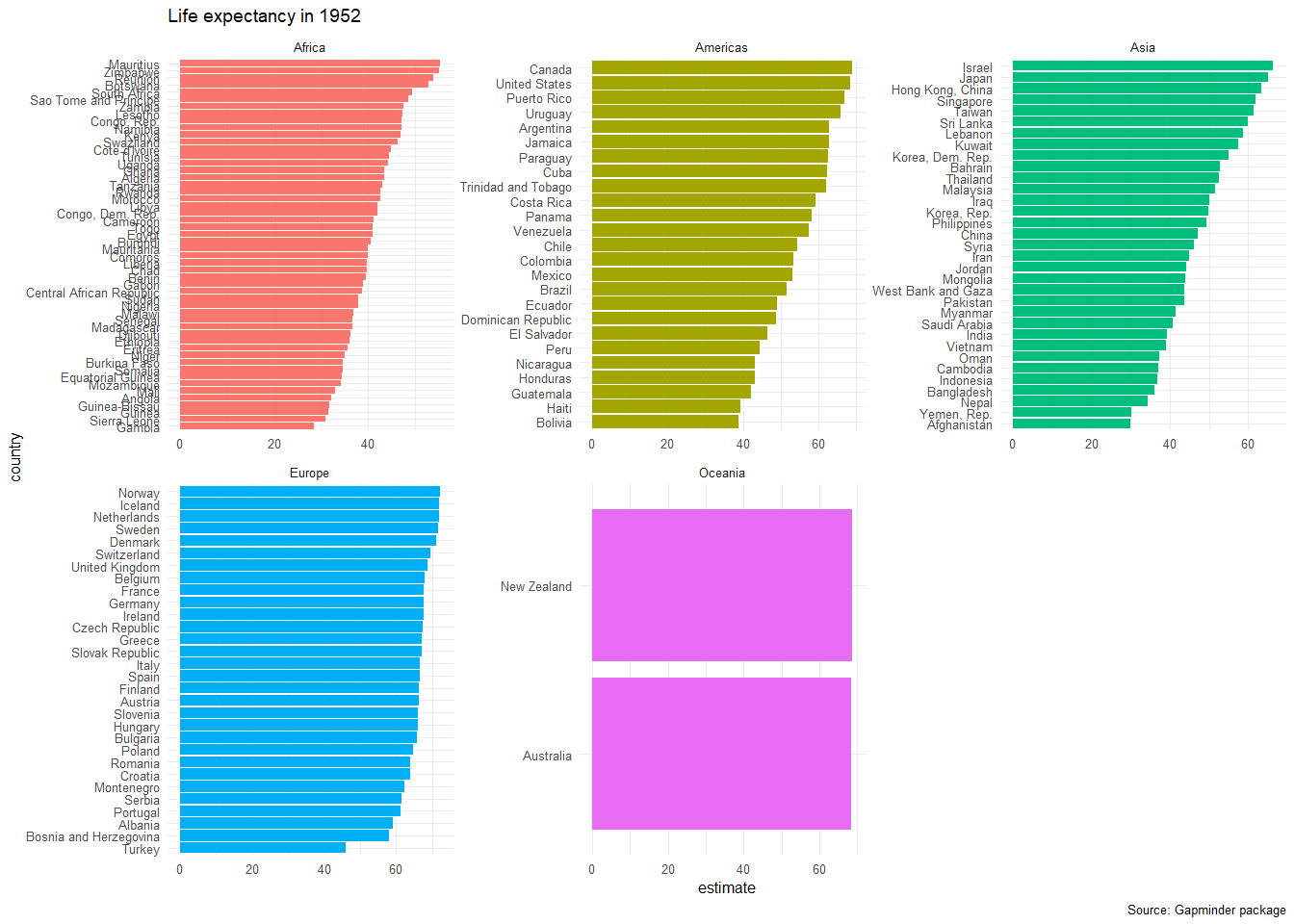
  ggplot(data = slopes, aes(x = country, y = estimate, fill = continent))+
  geom_col()+
  coord_flip()+
  theme_minimal(6)+
  facet_wrap(~continent, scales="free")+
  labs(title = 'Average yearly improvement in life expectancy, 1952-2007',
       caption = 'Source: Gapminder package') +
  theme(legend.position="none")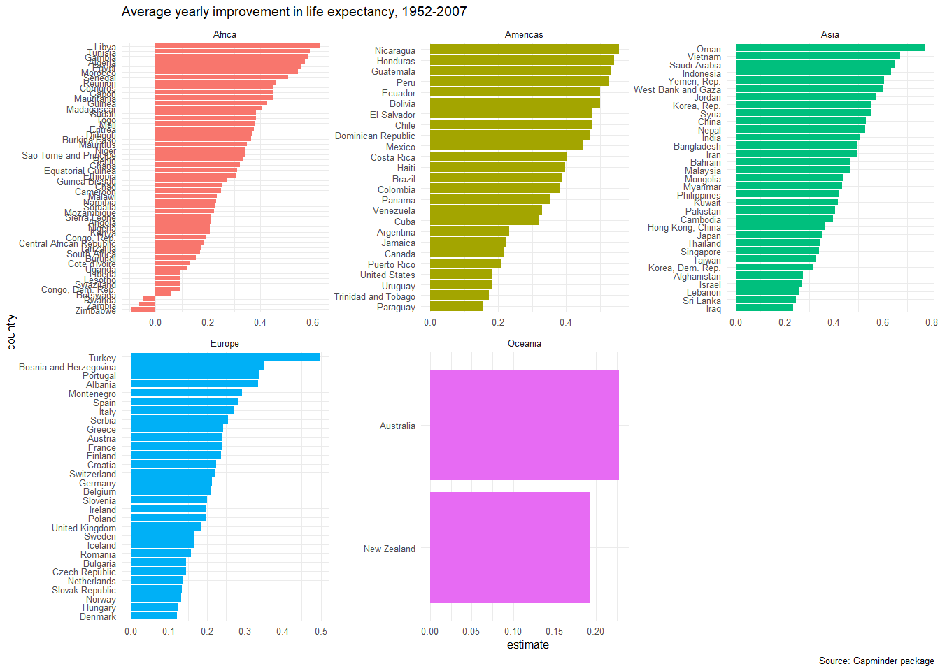
Finally, as in every regression model, the slopes are estimates for the yearly improvement in life expectancy. If we wanted to, we can plot the confidence interval for each country’s improvement.
  ggplot(data = slopes, aes(x = country, y = estimate, colour = continent))+
  geom_pointrange(aes(ymin = conf.low, ymax = conf.high))+
  coord_flip()+
  theme_minimal(6)+
  facet_wrap(~continent, scales="free")+
  labs(title = 'Average yearly improvement in life expectancy, 1952-2007',
       caption = 'Source: Gapminder package') +
  theme(legend.position="none")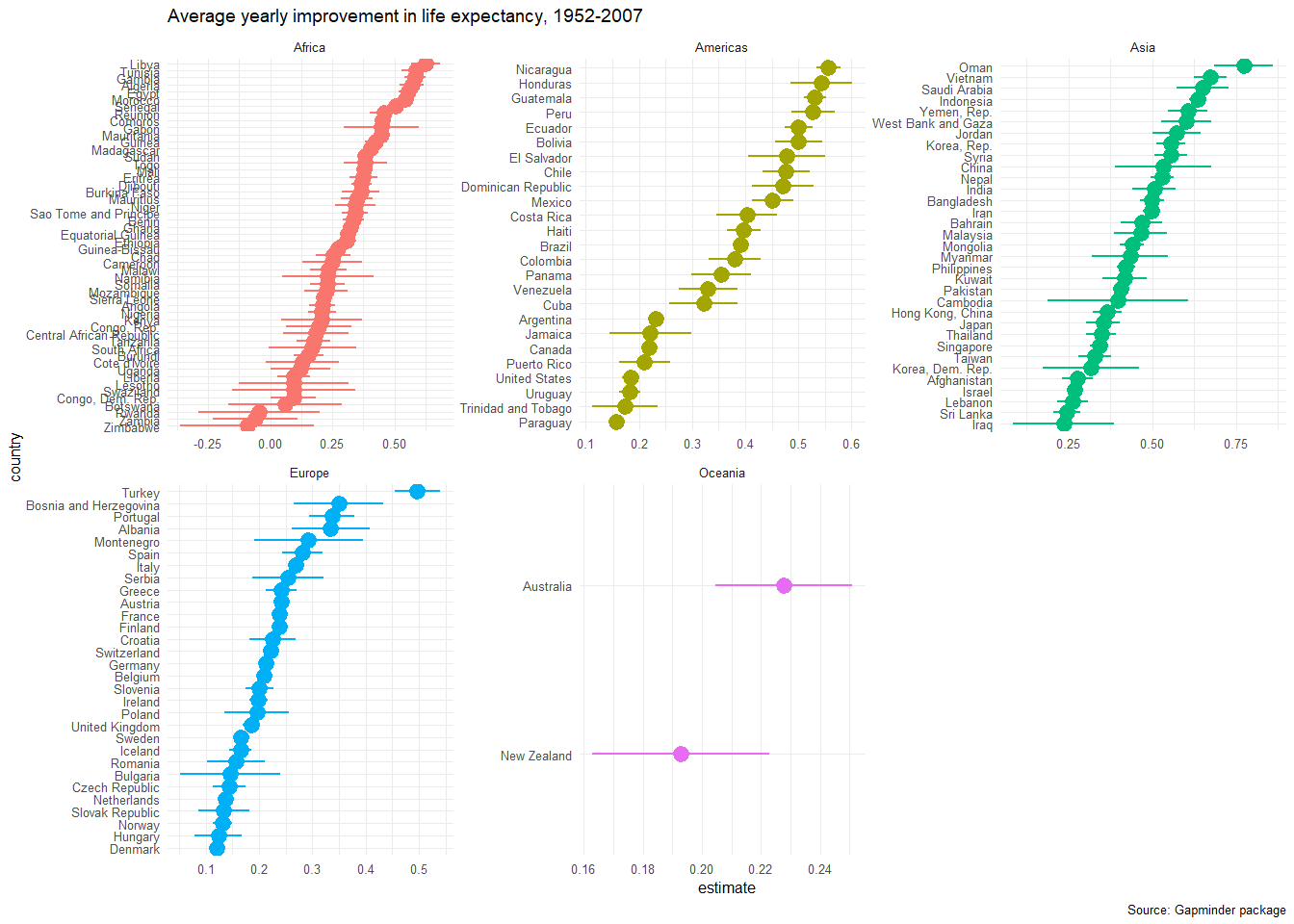
11.3 Further Resources
This page last updated on: 2020-07-14