16. Scraping web data
16.1 Overview
In few cases, one can find CSV or other type of flat files available on the internet. However, most of the times the data is not organised into a file that you can directly download into R. In these cases, we must use an Application Programming Interface (API), a description of the requests that can be sent to a certain service (database, website, etc.) and the kind of data that are returned. Many sources of data have made their data available via APIs over the internet; a computer program, or client, can make requests to the server, and the server responds back with the data, or with an error message.
16.2 Registering your API
We have seen the functionality of some packages,tidyverse, wbstats, eurostat) that provide API wrappers and make life easier. However, there are many cases where you would like to get data or use a service with an API query when no ready-made R package exists. In addition, one can also scape data off a website, such as tables that appear in a Wikipedia entry or download someone’s tweets; we will be looking at this in another section.
Many APIs require you to register for access. This allows them to track who is querying their services and, more importantly, to manage demand - if you submit too many queries too quickly, you might be rate-limited and your requests de-prioritized or blocked. You should always check the API access policy of the web site to determine what these limits are.
Let us consider an example. Opencagedata provides an API to geocode, namely to convert back and forth between geographical coordinates (longitude/latitude) and addresses. I actually believe this is a better geocoder than the one used in Google maps.
In order to be able to use their service you must: - install the package with: install.packages("opencage") - Go to the opencage website and sign up for an account. Make sure you select both forward and reverse geocoding. -By default you get the free service that allows 2,500 requests/day and limits you to 1 request/sec. - Once you register, you get an email with your API key, or you can go to the dashboard and be able to see and copy your API key there.
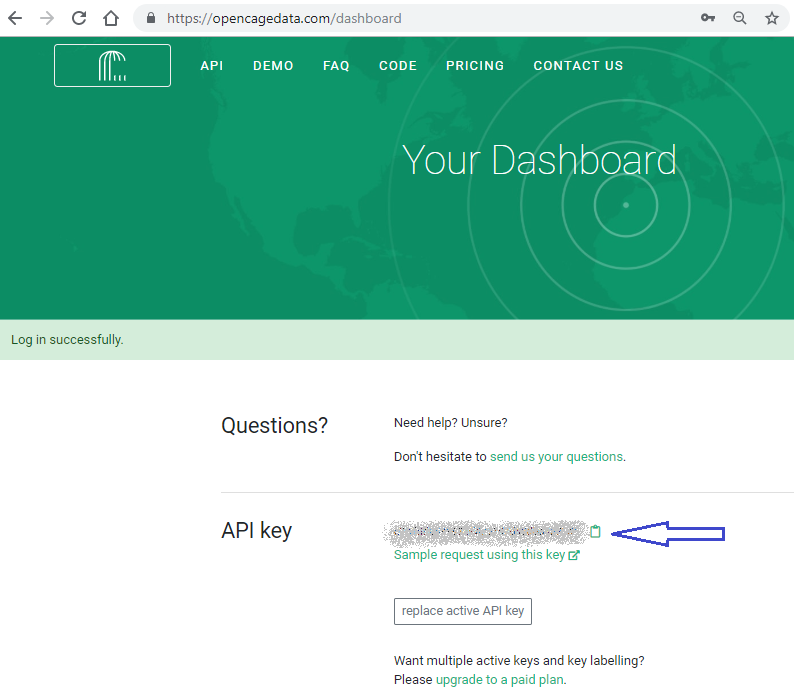
All functions of the opencage package will conveniently look for your API key, so before using the service, you must save your API key as an R environment variable, rather than having to input it manually in every single function call.
To save your API key, you must create (or edit) a file, .Renviron; this is a hidden file that lives in your home directory. The easiest way to find and edit .Renviron is with a function from the usethis package. In R, after you load the usethis package with library(usethis) you just invoke
usethis::edit_r_environ()
Your .Renviron file should show up in your editor, where you add a line
OPENCAGE_KEY=“xxxxxxxxxxxxxxxxxxxxxxxxxxxxxxx”
with your own, unique API key.
Before you exit, make sure your .Renviron ends with a blank line, then save and close it. Restart RStudio after modifying .Renviron in order to load the API key into memory. To check everything worked, go to console and type Sys.getenv("OPENCAGE_KEY")
Now that we have set the API key as an environment variable, we can geocode the LBS postcode using opencage_forward(). The results we get are not just the latitude/longitude coordinates that allow us to pinpoint NW1 4SA on a map, but a wealth of other information.
We can also use opencage_reverse(), where we pass the latitude/longitude coordinates, and, in our example, we get back information on Soho’s John Snow pub (and no, there is no pub named after the fictional Jon Snow).
library(opencage)

# Forward geocode London Business School postcode, NW1 4SA.
lbs_geocode <- opencage_forward("NW1 4SA")
lbs_geocode$results %>%
  knitr::kable() %>%
  kable_styling(c("striped", "bordered")) %>%
scroll_box(width = "100%", height = "200px")| annotations.DMS.lat | annotations.DMS.lng | annotations.MGRS | annotations.Maidenhead | annotations.Mercator.x | annotations.Mercator.y | annotations.OSM.note_url | annotations.OSM.url | annotations.UN_M49.regions.EUROPE | annotations.UN_M49.regions.GB | annotations.UN_M49.regions.NORTHERN_EUROPE | annotations.UN_M49.regions.WORLD | annotations.UN_M49.statistical_groupings | annotations.callingcode | annotations.currency.decimal_mark | annotations.currency.html_entity | annotations.currency.iso_code | annotations.currency.iso_numeric | annotations.currency.name | annotations.currency.smallest_denomination | annotations.currency.subunit | annotations.currency.subunit_to_unit | annotations.currency.symbol | annotations.currency.symbol_first | annotations.currency.thousands_separator | annotations.flag | annotations.geohash | annotations.qibla | annotations.roadinfo.drive_on | annotations.roadinfo.speed_in | annotations.sun.rise.apparent | annotations.sun.rise.astronomical | annotations.sun.rise.civil | annotations.sun.rise.nautical | annotations.sun.set.apparent | annotations.sun.set.astronomical | annotations.sun.set.civil | annotations.sun.set.nautical | annotations.timezone.name | annotations.timezone.now_in_dst | annotations.timezone.offset_sec | annotations.timezone.offset_string | annotations.timezone.short_name | annotations.what3words.words | components.ISO_3166-1_alpha-2 | components.ISO_3166-1_alpha-3 | components._category | components._type | components.city | components.continent | components.country | components.country_code | components.county | components.county_code | components.postcode | components.state | components.state_code | components.suburb | confidence | formatted | geometry.lat | geometry.lng | query |
|---|---|---|---|---|---|---|---|---|---|---|---|---|---|---|---|---|---|---|---|---|---|---|---|---|---|---|---|---|---|---|---|---|---|---|---|---|---|---|---|---|---|---|---|---|---|---|---|---|---|---|---|---|---|---|---|---|---|---|---|---|---|---|
| 51° 31’ 35.69160’’ N | 0° 9’ 40.96080’’ E | 30UXC9690312205 | IO91wm06pj | -17964.517 | 6681500.038 | https://www.openstreetmap.org/note/new#map=16/51.52658/-0.16138&layers=N | https://www.openstreetmap.org/?mlat=51.52658&mlon=-0.16138#map=16/51.52658/-0.16138 | 150 | 826 | 154 | 001 | MEDC | 44 | . | £ | GBP | 826 | British Pound | 1 | Penny | 100 | £ | 1 | , | <U+0001F1EC><U+0001F1E7> | gcpvhk4kpdgu4uvu403f | 118.97 | left | mph | 1594699320 | 0 | 1594696620 | 1594692720 | 1594757460 | 0 | 1594760100 | 1594764000 | Europe/London | 1 | 3600 | +0100 | BST | humans.unit.volume | GB | GBR | postcode | postcode | London | Europe | United Kingdom | gb | Westminster | WSM | NW1 4SA | England | ENG | Regent’s Park | 10 | London NW1 4SA, United Kingdom | 51.5 | -0.161 | NW1 4SA |
# Reverse geocode latitude/longitude that corresponds
# to the The John Snow pub in 39 Browadwick Street, Soho, London
reverse_john_snow <- opencage_reverse(51.51328, -0.13657)
reverse_john_snow$results %>%
  knitr::kable() %>%
  kable_styling(c("striped", "bordered")) %>%
scroll_box(width = "100%", height = "200px")| annotations.DMS.lat | annotations.DMS.lng | annotations.MGRS | annotations.Maidenhead | annotations.Mercator.x | annotations.Mercator.y | annotations.OSM.edit_url | annotations.OSM.note_url | annotations.OSM.url | annotations.UN_M49.regions.EUROPE | annotations.UN_M49.regions.GB | annotations.UN_M49.regions.NORTHERN_EUROPE | annotations.UN_M49.regions.WORLD | annotations.UN_M49.statistical_groupings | annotations.callingcode | annotations.currency.decimal_mark | annotations.currency.html_entity | annotations.currency.iso_code | annotations.currency.iso_numeric | annotations.currency.name | annotations.currency.smallest_denomination | annotations.currency.subunit | annotations.currency.subunit_to_unit | annotations.currency.symbol | annotations.currency.symbol_first | annotations.currency.thousands_separator | annotations.flag | annotations.geohash | annotations.qibla | annotations.roadinfo.drive_on | annotations.roadinfo.road | annotations.roadinfo.speed_in | annotations.sun.rise.apparent | annotations.sun.rise.astronomical | annotations.sun.rise.civil | annotations.sun.rise.nautical | annotations.sun.set.apparent | annotations.sun.set.astronomical | annotations.sun.set.civil | annotations.sun.set.nautical | annotations.timezone.name | annotations.timezone.now_in_dst | annotations.timezone.offset_sec | annotations.timezone.offset_string | annotations.timezone.short_name | annotations.what3words.words | bounds.northeast.lat | bounds.northeast.lng | bounds.southwest.lat | bounds.southwest.lng | components.ISO_3166-1_alpha-2 | components.ISO_3166-1_alpha-3 | components._category | components._type | components.city | components.continent | components.country | components.country_code | components.county | components.county_code | components.house_number | components.postcode | components.pub | components.road | components.state | components.state_code | components.state_district | components.suburb | confidence | formatted | geometry.lat | geometry.lng | query |
|---|---|---|---|---|---|---|---|---|---|---|---|---|---|---|---|---|---|---|---|---|---|---|---|---|---|---|---|---|---|---|---|---|---|---|---|---|---|---|---|---|---|---|---|---|---|---|---|---|---|---|---|---|---|---|---|---|---|---|---|---|---|---|---|---|---|---|---|---|---|---|---|---|
| 51° 30’ 47.79864’’ N | 0° 8’ 11.73588’’ E | 30UXC9868010793 | IO91wm33oe | -15205.495 | 6679126.202 | https://www.openstreetmap.org/edit?way=273697641#map=16/51.51328/-0.13659 | https://www.openstreetmap.org/note/new#map=16/51.51328/-0.13659&layers=N | https://www.openstreetmap.org/?mlat=51.51328&mlon=-0.13659#map=16/51.51328/-0.13659 | 150 | 826 | 154 | 001 | MEDC | 44 | . | £ | GBP | 826 | British Pound | 1 | Penny | 100 | £ | 1 | , | <U+0001F1EC><U+0001F1E7> | gcpvhcsw94usv1nxc7x6 | 118.98 | left | Broadwick Street | mph | 1594699320 | 0 | 1594696620 | 1594692720 | 1594757460 | 0 | 1594760100 | 1594764000 | Europe/London | 1 | 3600 | +0100 | BST | tests.exist.rungs | 51.5133344 | -0.1365051 | 51.5132212 | -0.136682 | GB | GBR | commerce | pub | London | Europe | United Kingdom | gb | Westminster | WSM | 39 | W1F 9QJ | The John Snow | Broadwick Street | England | ENG | Greater London | Soho | 9 | The John Snow, 39 Broadwick Street, London W1F 9QJ, United Kingdom | 51.5 | -0.137 | 51.51328,-0.13657 |
16.3 rtweet: Twitter data and Text Mining
The rtweet package allows us to download Twitter data. Besides having your own Twitter account, you must create a Twitter app in order to get a Twitter API access token. To do this,
- Login in in your Twitter account, and go to https://developer.twitter.com/en/apps/create
- Create a new app by providing a name, description, and website as shown below. Also, please add a short description towards the end of what you plan to do (text analysis, plotting, etc).
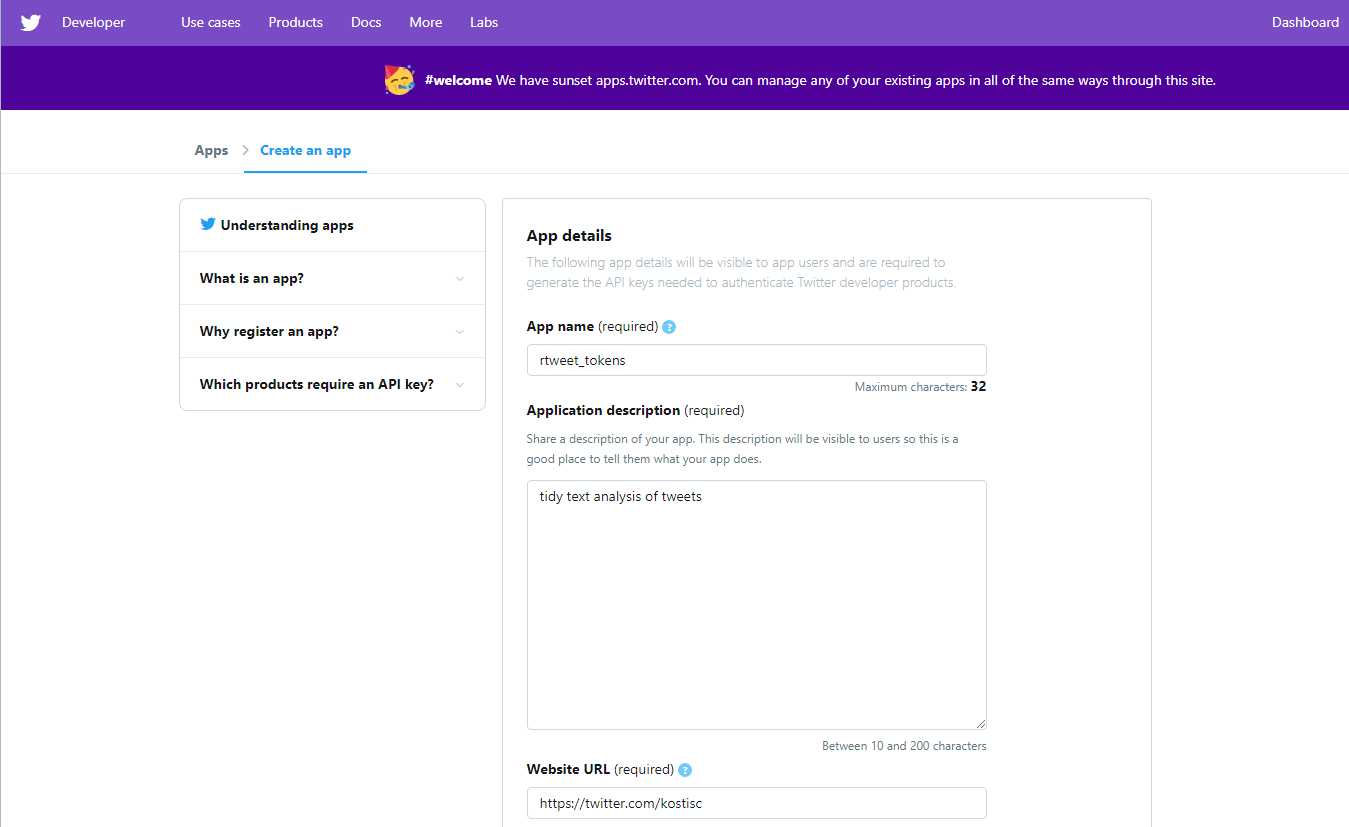
Once you create your application and it’s approved, go to the Keys and Tokens tab, and find the values Consumer Key (aka “API Key”) and Consumer Secret (aka “API Secret”).
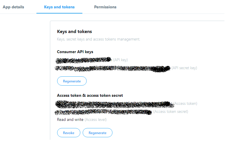
Copy and paste the two keys (along with the name of your app) into an R script file and pass them along to create_token(), using your own keys, rather than xxxx.
## autheticate via web browser
token <- create_token(
  app = "rtweet_tokens",
  consumer_key = "xxxxxxxxxxxxxxxx",
  consumer_secret = "xxxxxxxxxxxxxxxx",
  access_token  = "xxxxxxxxxxxxxxxx",
  access_secret  = "xxxxxxxxxxxxxxxx")
A browser window should pop up. If you are logged in your Twitter account, click to approve and return to R. The rtweet::create_token() function should automatically save your token as an environment variable for you. To make sure it worked, compare the created token object to the object returned by rtweet::get_token()
16.3.1 Text Mining
Now that you have authorised the Twitter API, let us retrieve the most recent 3200 tweets of a couple of Twitter users who appear to be friends](https://twitter.com/realDonaldTrump/status/1001961235838103552), Sesame Street’s Cookie Monster, and the BBC Breaking News service. For all users, we will plot their weekly tweet frequency, and perform a text mining analysis.
# load twitter library
library(rtweet)

# plotting and pipes and dplyr - tidyverse
library(tidyverse)

# text mining
library(tidytext)
library(textdata)

# retrieve most recent 3200 tweets of some twitter users- this is the max we can retrieve
twitter_users <- get_timeline(
  user = c("BBCBreaking", "KimKardashian", "MeCookieMonster", "realDonaldTrump"),
  n = 3200
)

# group by user and plot weekly tweet frequency
twitter_users %>%
  group_by(screen_name) %>%
  ts_plot(by = "months")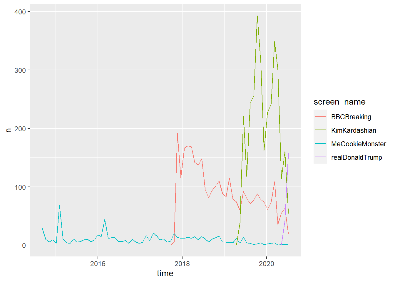
Some lines seem to stop earlier; it’s not there was no activity before that, but this shows that some users are busier tweeting than others; Donald Trump has been busier tweeting and his last 3200 tweets cover just a few months, compared to others.
It would be interesting to do a quick text mining analysis; Let us first glimpse at the dataframe, to see its structure, variables names, etc.
## Rows: 7,295
## Columns: 90
## $ user_id                 <chr> "5402612", "5402612", "5402612", "5402612",...
## $ status_id               <chr> "1283020124220514305", "1283005301508255745...
## $ created_at              <dttm> 2020-07-14 12:46:49, 2020-07-14 11:47:55, ...
## $ screen_name             <chr> "BBCBreaking", "BBCBreaking", "BBCBreaking"...
## $ text                    <chr> "US government puts to death man who killed...
## $ source                  <chr> "TweetDeck", "TweetDeck", "SocialFlow", "So...
## $ display_text_width      <dbl> 124, 125, 110, 165, 111, 132, 116, 140, 142...
## $ reply_to_status_id      <chr> "1282929825947279360", NA, NA, NA, NA, NA, ...
## $ reply_to_user_id        <chr> "5402612", NA, NA, NA, NA, NA, NA, NA, NA, ...
## $ reply_to_screen_name    <chr> "BBCBreaking", NA, NA, NA, NA, NA, NA, NA, ...
## $ is_quote                <lgl> FALSE, FALSE, FALSE, FALSE, FALSE, FALSE, F...
## $ is_retweet              <lgl> FALSE, FALSE, FALSE, FALSE, FALSE, FALSE, F...
## $ favorite_count          <int> 973, 5899, 1582, 936, 3524, 12208, 3490, 0,...
## $ retweet_count           <int> 206, 2339, 476, 353, 999, 3866, 1499, 1015,...
## $ quote_count             <int> NA, NA, NA, NA, NA, NA, NA, NA, NA, NA, NA,...
## $ reply_count             <int> NA, NA, NA, NA, NA, NA, NA, NA, NA, NA, NA,...
## $ hashtags                <list> [NA, NA, NA, NA, NA, NA, NA, NA, NA, NA, N...
## $ symbols                 <list> [NA, NA, NA, NA, NA, NA, NA, NA, NA, NA, N...
## $ urls_url                <list> ["bbc.in/392pRRa", "bbc.in/396b489", "bbc....
## $ urls_t.co               <list> ["https://t.co/vEQL9jy50o", "https://t.co/...
## $ urls_expanded_url       <list> ["https://bbc.in/392pRRa", "https://bbc.in...
## $ media_url               <list> [NA, NA, NA, NA, NA, NA, NA, NA, NA, NA, N...
## $ media_t.co              <list> [NA, NA, NA, NA, NA, NA, NA, NA, NA, NA, N...
## $ media_expanded_url      <list> [NA, NA, NA, NA, NA, NA, NA, NA, NA, NA, N...
## $ media_type              <list> [NA, NA, NA, NA, NA, NA, NA, NA, NA, NA, N...
## $ ext_media_url           <list> [NA, NA, NA, NA, NA, NA, NA, NA, NA, NA, N...
## $ ext_media_t.co          <list> [NA, NA, NA, NA, NA, NA, NA, NA, NA, NA, N...
## $ ext_media_expanded_url  <list> [NA, NA, NA, NA, NA, NA, NA, NA, NA, NA, N...
## $ ext_media_type          <chr> NA, NA, NA, NA, NA, NA, NA, NA, NA, NA, NA,...
## $ mentions_user_id        <list> [NA, NA, NA, NA, NA, NA, NA, "265902729", ...
## $ mentions_screen_name    <list> [NA, NA, NA, NA, NA, NA, NA, "BBCSport", N...
## $ lang                    <chr> "en", "en", "en", "en", "en", "en", "en", "...
## $ quoted_status_id        <chr> NA, NA, NA, NA, NA, NA, NA, NA, NA, NA, NA,...
## $ quoted_text             <chr> NA, NA, NA, NA, NA, NA, NA, NA, NA, NA, NA,...
## $ quoted_created_at       <dttm> NA, NA, NA, NA, NA, NA, NA, NA, NA, NA, NA...
## $ quoted_source           <chr> NA, NA, NA, NA, NA, NA, NA, NA, NA, NA, NA,...
## $ quoted_favorite_count   <int> NA, NA, NA, NA, NA, NA, NA, NA, NA, NA, NA,...
## $ quoted_retweet_count    <int> NA, NA, NA, NA, NA, NA, NA, NA, NA, NA, NA,...
## $ quoted_user_id          <chr> NA, NA, NA, NA, NA, NA, NA, NA, NA, NA, NA,...
## $ quoted_screen_name      <chr> NA, NA, NA, NA, NA, NA, NA, NA, NA, NA, NA,...
## $ quoted_name             <chr> NA, NA, NA, NA, NA, NA, NA, NA, NA, NA, NA,...
## $ quoted_followers_count  <int> NA, NA, NA, NA, NA, NA, NA, NA, NA, NA, NA,...
## $ quoted_friends_count    <int> NA, NA, NA, NA, NA, NA, NA, NA, NA, NA, NA,...
## $ quoted_statuses_count   <int> NA, NA, NA, NA, NA, NA, NA, NA, NA, NA, NA,...
## $ quoted_location         <chr> NA, NA, NA, NA, NA, NA, NA, NA, NA, NA, NA,...
## $ quoted_description      <chr> NA, NA, NA, NA, NA, NA, NA, NA, NA, NA, NA,...
## $ quoted_verified         <lgl> NA, NA, NA, NA, NA, NA, NA, NA, NA, NA, NA,...
## $ retweet_status_id       <chr> NA, NA, NA, NA, NA, NA, NA, "12825949926960...
## $ retweet_text            <chr> NA, NA, NA, NA, NA, NA, NA, "Manchester Cit...
## $ retweet_created_at      <dttm> NA, NA, NA, NA, NA, NA, NA, 2020-07-13 08:...
## $ retweet_source          <chr> NA, NA, NA, NA, NA, NA, NA, "TweetDeck", NA...
## $ retweet_favorite_count  <int> NA, NA, NA, NA, NA, NA, NA, 3990, NA, 4014,...
## $ retweet_retweet_count   <int> NA, NA, NA, NA, NA, NA, NA, 1015, NA, 820, ...
## $ retweet_user_id         <chr> NA, NA, NA, NA, NA, NA, NA, "265902729", NA...
## $ retweet_screen_name     <chr> NA, NA, NA, NA, NA, NA, NA, "BBCSport", NA,...
## $ retweet_name            <chr> NA, NA, NA, NA, NA, NA, NA, "BBC Sport", NA...
## $ retweet_followers_count <int> NA, NA, NA, NA, NA, NA, NA, 8465538, NA, 84...
## $ retweet_friends_count   <int> NA, NA, NA, NA, NA, NA, NA, 326, NA, 326, N...
## $ retweet_statuses_count  <int> NA, NA, NA, NA, NA, NA, NA, 468003, NA, 468...
## $ retweet_location        <chr> NA, NA, NA, NA, NA, NA, NA, "MediaCityUK, S...
## $ retweet_description     <chr> NA, NA, NA, NA, NA, NA, NA, "Official https...
## $ retweet_verified        <lgl> NA, NA, NA, NA, NA, NA, NA, TRUE, NA, TRUE,...
## $ place_url               <chr> NA, NA, NA, NA, NA, NA, NA, NA, NA, NA, NA,...
## $ place_name              <chr> NA, NA, NA, NA, NA, NA, NA, NA, NA, NA, NA,...
## $ place_full_name         <chr> NA, NA, NA, NA, NA, NA, NA, NA, NA, NA, NA,...
## $ place_type              <chr> NA, NA, NA, NA, NA, NA, NA, NA, NA, NA, NA,...
## $ country                 <chr> NA, NA, NA, NA, NA, NA, NA, NA, NA, NA, NA,...
## $ country_code            <chr> NA, NA, NA, NA, NA, NA, NA, NA, NA, NA, NA,...
## $ geo_coords              <list> [<NA, NA>, <NA, NA>, <NA, NA>, <NA, NA>, <...
## $ coords_coords           <list> [<NA, NA>, <NA, NA>, <NA, NA>, <NA, NA>, <...
## $ bbox_coords             <list> [<NA, NA, NA, NA, NA, NA, NA, NA>, <NA, NA...
## $ status_url              <chr> "https://twitter.com/BBCBreaking/status/128...
## $ name                    <chr> "BBC Breaking News", "BBC Breaking News", "...
## $ location                <chr> "London, UK", "London, UK", "London, UK", "...
## $ description             <chr> "Breaking news alerts and updates from the ...
## $ url                     <chr> "http://t.co/vBzl7LOaso", "http://t.co/vBzl...
## $ protected               <lgl> FALSE, FALSE, FALSE, FALSE, FALSE, FALSE, F...
## $ followers_count         <int> 44557304, 44557304, 44557304, 44557304, 445...
## $ friends_count           <int> 3, 3, 3, 3, 3, 3, 3, 3, 3, 3, 3, 3, 3, 3, 3...
## $ listed_count            <int> 135627, 135627, 135627, 135627, 135627, 135...
## $ statuses_count          <int> 36640, 36640, 36640, 36640, 36640, 36640, 3...
## $ favourites_count        <int> 0, 0, 0, 0, 0, 0, 0, 0, 0, 0, 0, 0, 0, 0, 0...
## $ account_created_at      <dttm> 2007-04-22 14:42:37, 2007-04-22 14:42:37, ...
## $ verified                <lgl> TRUE, TRUE, TRUE, TRUE, TRUE, TRUE, TRUE, T...
## $ profile_url             <chr> "http://t.co/vBzl7LOaso", "http://t.co/vBzl...
## $ profile_expanded_url    <chr> "http://www.bbc.co.uk/news", "http://www.bb...
## $ account_lang            <lgl> NA, NA, NA, NA, NA, NA, NA, NA, NA, NA, NA,...
## $ profile_banner_url      <chr> "https://pbs.twimg.com/profile_banners/5402...
## $ profile_background_url  <chr> "http://abs.twimg.com/images/themes/theme1/...
## $ profile_image_url       <chr> "http://pbs.twimg.com/profile_images/115071...
Text mining is essentially a neat way to count words, calculate their frequency, and map words into sentiments using a sentiment analysis lexicon. The results of text mining seems impressive, but it isn’t magic — it’s really just counting.
The first step in text mining is to take text and tokenise it, namely to take whatever is written and turn it into a word-by-word column. In addition, when we process text, we filter out the most common words in a language; these are called stop words, for example and, but, the, is, at, etc.
In our case, there are 90 variables (or columns), and we just to want to concentrate on what users wrote, rather than retweeted (is_retweet). We will use dplyr to filter out retweets and then use tidytext::unnest_tokens() to split a sentence into one-word-per-column, as shown below.
tidy_tweets <- twitter_users %>% # #take the data frame, and then
  filter(is_retweet==FALSE)%>% # filter just their original tweets, and then
  select(screen_name, text)%>% # select variables of interest, and then
  unnest_tokens(word, text) # split column with text in one word (or token)-per-row format

tidy_tweets %>% #take the data frame, and then
  filter(screen_name == "realDonaldTrump") %>%#filter tweets for a certain user
  head(20) %>% #show the first 20 rows, and then
  knitr::kable() %>% # use kable to make the table look good
kable_styling(c("striped", "bordered")) | screen_name | word |
|---|---|
| realDonaldTrump | would |
| realDonaldTrump | be |
| realDonaldTrump | so |
| realDonaldTrump | great |
| realDonaldTrump | if |
| realDonaldTrump | the |
| realDonaldTrump | media |
| realDonaldTrump | would |
| realDonaldTrump | get |
| realDonaldTrump | the |
| realDonaldTrump | word |
| realDonaldTrump | out |
| realDonaldTrump | to |
| realDonaldTrump | the |
| realDonaldTrump | people |
| realDonaldTrump | in |
| realDonaldTrump | a |
| realDonaldTrump | fair |
| realDonaldTrump | and |
| realDonaldTrump | balanced |
Reading text like this is very unwiedly for human, but very efficient for computers, as we can easily group them, count them, etc.
As we mentiond earlier, when we process text, we filter out the most common words used in a language; these are called stop words, for example and, but, the, is, at, etc., and below we can see the first few entries for such stop words.
stop_words %>% #take the stop_words, and then
  head(20) %>% #show the first 20 rows, and then
  knitr::kable() %>% #make the table better looking
kable_styling(c("striped", "bordered")) | word | lexicon |
|---|---|
| a | SMART |
| a’s | SMART |
| able | SMART |
| about | SMART |
| above | SMART |
| according | SMART |
| accordingly | SMART |
| across | SMART |
| actually | SMART |
| after | SMART |
| afterwards | SMART |
| again | SMART |
| against | SMART |
| ain’t | SMART |
| all | SMART |
| allow | SMART |
| allows | SMART |
| almost | SMART |
| alone | SMART |
| along | SMART |
In addition to these stop words, we should create another set of stop words specific to Twitter– these are words that include https for webpage addresses, rt for retweet, t.co which is a URL shorthand notation, etc.
twitter_stop_words <- tibble( #construct a dataframe
  word = c(
    "https",
    "t.co",
    "rt",
    "amp"
  ),
  lexicon = "twitter"
)
# Connect stop words
all_stop_words <- stop_words %>%
  bind_rows(twitter_stop_words) # connect two data frames row-wise

# Remove numbers
no_numbers <- tidy_tweets %>%
    filter(is.na(as.numeric(word))) # filter() returns rows where conditions are true
So far, we have defined our stop words and got rid of tweets that contain numbers. We will now use anti_join() to get rid of all stop words in our dataframe. anti_join() returns all rows from the dataframe where there are not matching values that are contained in all_stop_words.
# Get rid of the combined stop words by using anti_join().
# anti_join() returns all rows from x where there are not matching values in y

no_stop_words <- no_numbers %>%
  anti_join(all_stop_words, by = "word")

# instead of anti_join() we could also use
# filter(!(word %in% all_stop_words$word))

no_stop_words <- no_numbers %>%
  filter(!(word %in% all_stop_words$word))

# We group by screen_name, and then
# count and sort number of times each word appears, and then
# sort the list, and then
# keep the top 20 words

words_count<- no_stop_words %>%
  dplyr::group_by(screen_name) %>%
  dplyr::count(word, sort = TRUE) %>%
  top_n(20) %>%
  ungroup()
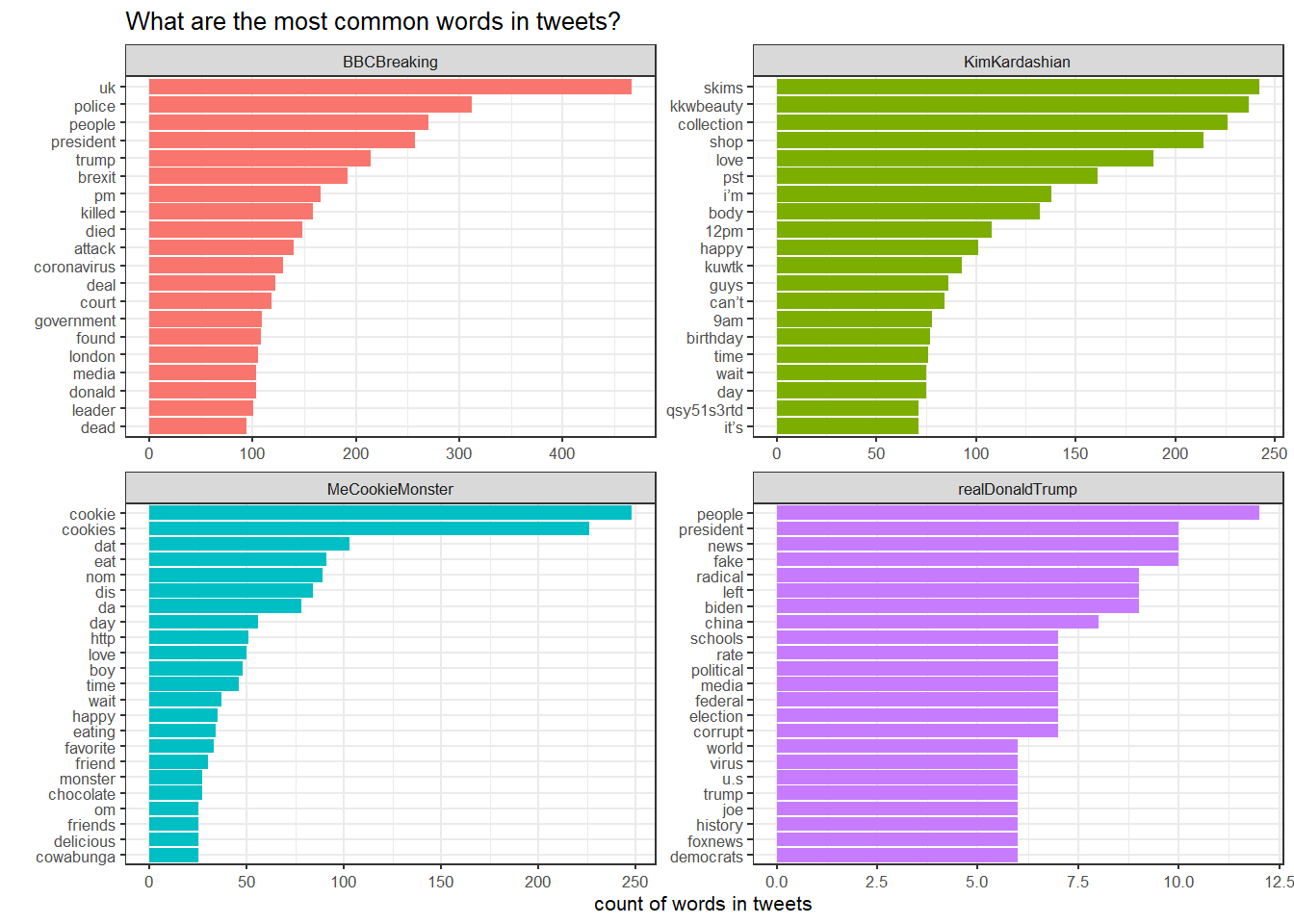
The great majority of tweeted words is stop words. Removing the stop words is important for visualisation and sentiment analysis - we only want to plot and analyse the top 25 interesting words for each user. This is a slightly trickier plot, as we have to get the top words per user. To do this, we shall use tidytext::reorder_within() with three arguments:
- the item we want to reorder, namely
word - what we want to reorder by; in our case
n, the number of times a word was used, and - the groups or categories we want to reorder within, in our case
screen_name
After we reorder_within, we used scale_x_reordered()to finish making this plot.
words_count %>%
  mutate(word = reorder_within(word, n, screen_name)) %>%
  ggplot(aes(x=word, y=n, fill = screen_name)) +
  geom_col(show.legend = FALSE) +
  facet_wrap(~screen_name, scales = "free") +
  coord_flip() +
  scale_x_reordered()+
  theme_bw(8)+
  labs(
    title = "What are the most common words in tweets?",
    x = "",
    y = "count of words in tweets"
) 
16.3.2 Frequency of pairs of words in tweets
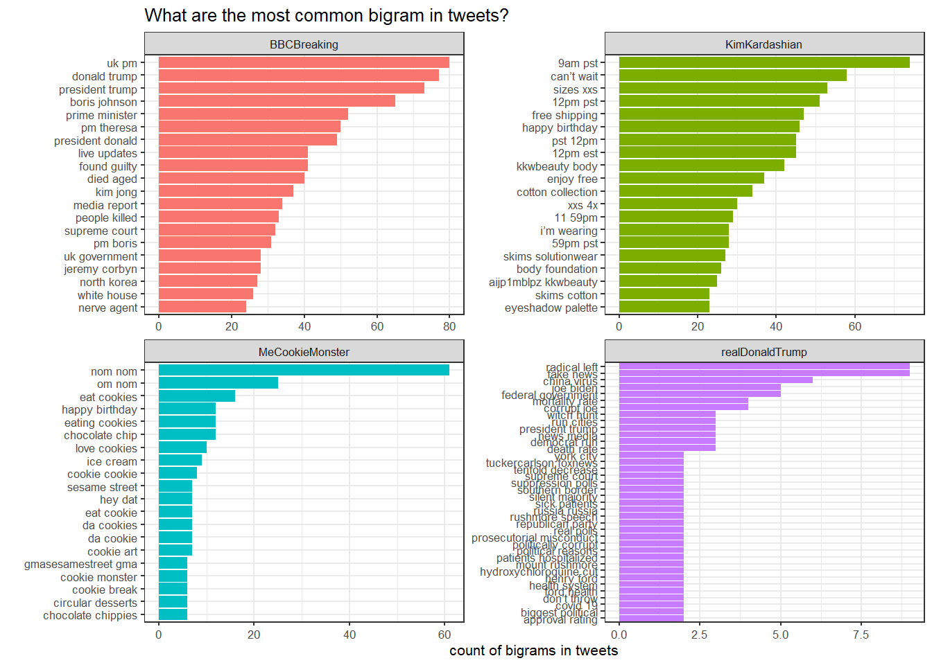
We can also look at the frequency of pairs of words, or bigrams, rather than looking at single words. We will look at common bigrams and again filter out stop words, as we do not want things like of, the, and, that, etc.
tweet_bigrams <- twitter_users %>% # #take the data frame, and then
  filter(is_retweet==FALSE)%>% # filter just their original tweets, and then
  select(screen_name, text)%>% # select variables of interest, and then

  # create column bigram with tweet text with n=2 words-per-row
  unnest_tokens(bigram, text, token = "ngrams", n = 2) %>%
  # Split the bigram column into two columns
  separate(bigram, c("word1", "word2"), sep = " ") %>%

  filter(!word1 %in% all_stop_words$word,
         !word2 %in% all_stop_words$word) %>%
  # Put the two word columns back together
  unite(bigram, word1, word2, sep = " ") %>%
  dplyr::group_by(screen_name) %>%
  dplyr::count(bigram, sort = TRUE) %>%
  top_n(20) %>%
  ungroup()


tweet_bigrams %>%
  mutate(bigram = reorder_within(bigram, n, screen_name)) %>%
  ggplot(aes(x=bigram, y=n, fill = screen_name)) +
  geom_col(show.legend = FALSE) +
  facet_wrap(~screen_name, scales = "free") +
  coord_flip() +
  scale_x_reordered()+
  theme_bw(8)+
  labs(
    title = "What are the most common bigram in tweets?",
    x = "",
    y = "count of bigrams in tweets"
) 
16.3.3 Sentiment Analysis
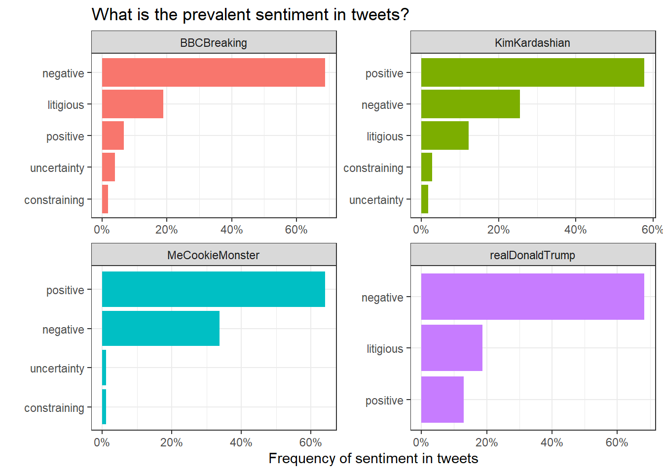
To perform sentiment analysis, we must use a specific sentiment lexicon that assigns individual words to different sentiments (negative, positive, uncertain, etc.)
sentiment <- get_sentiments("loughran") # get specific sentiment lexicon

sentiment_words <- no_stop_words %>%
  inner_join(sentiment, by="word")


sentiment_words %>%
  group_by(screen_name,sentiment) %>% # group by sentiment type
  summarise (n = n()) %>%
  mutate(freq = n / sum(n)) %>% #calculate frequency (%) of sentiments
  ungroup() %>%
  mutate(sentiment = reorder_within(sentiment, freq, screen_name)) %>%

  #and now plot the data
  ggplot(aes(x=sentiment, y=freq, fill = screen_name)) +
  geom_col(show.legend = FALSE) +
  scale_y_continuous(labels = scales::percent) +
  facet_wrap(~screen_name, scales = "free") +
  coord_flip() +
  theme_bw()+
  scale_x_reordered()+
  labs(
    title = "What is the prevalent sentiment in tweets?",
    x = "",
    y = "Frequency of sentiment in tweets"
) 
Finally, we can plot a world cloud, using the package wordcloud2 with the words that realDonaldTrump used the most.
library(wordcloud2)

# plot using wordcloud2

trump_word_count <- no_stop_words %>%
  filter(screen_name == 'realDonaldTrump') %>%
  dplyr::count(word, sort = TRUE) %>%
  top_n(500)


wordcloud2(trump_word_count)
16.4 rvest: scrape web data
This is a placeholder. Material on scraping web pages will appear here
16.5 Further Resources
16.6 Acknowledgments
This page last updated on: 2020-07-14