9. Reshape data with tidyr
9.1 Overview
It is often said that the vast majority of data analysis is spent on cleaning and preparing data. This is something that must be repeated many times over the course of analysis as new problems come to light or new data is collected.
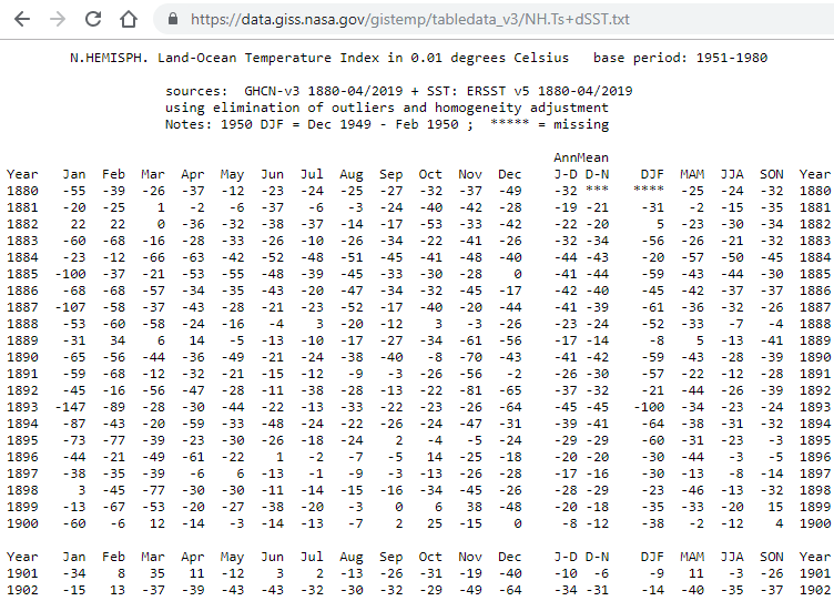
Most people are used to analyze data in a spreadsheet or tabular format. For instance, if we wanted to study climate change, we can find data on the Combined Land-Surface Air and Sea-Surface Water Temperature Anomalies in the Northern Hemisphere at NASA’s Goddard Institute for Space Studies. The tabular data of temperature anomalies can be found here and part of that data set is shown below:

A lot of these tabular shape spreadsheets were designed for efficient data entry and not necessarily to undertake any kind of statistical analysis. The principles of tidy data provide a standard way to organise data values within a dataset. A standard makes initial data cleaning easier because you don’t need to start from scratch and reinvent the wheel every time.
Tidy data is a specific way of organising data in a consistent manner and structuring datasets to facilitate analysis with the tidyverse. The tidy data standard has been designed to facilitate exploratory data analysis; tidy datasets and tidy tools help make data analysis easier, allowing you to focus on the interesting domain problem, not on the logistics of cleaning data.
Before we proceed, a few definitions taken from Garret Grolemund and the vignette(“tidy-data”)
- Variable: A quantity, quality, or property that you can measure.
- Observation: A set of values that display the relationship between variables. To be an observation, values need to be measured under similar conditions, usually measured on the same observational unit at the same time.
- Value: The state of a variable that you observe when you measure it.
There are three rules which make a dataset tidy:
- Each variable must have its own column.
- Each observation must have its own row.
- Each value must have its own cell.

Figure 12.1 from R for Data Science
A tidy dataset is a long dataset, where each variable appears in one column, and each observation has its own row. The weather anomalies dataset is a wide dataset; the three variables are date (or year and month if you wanted to keep them separate), and delta (the actual temperature difference).
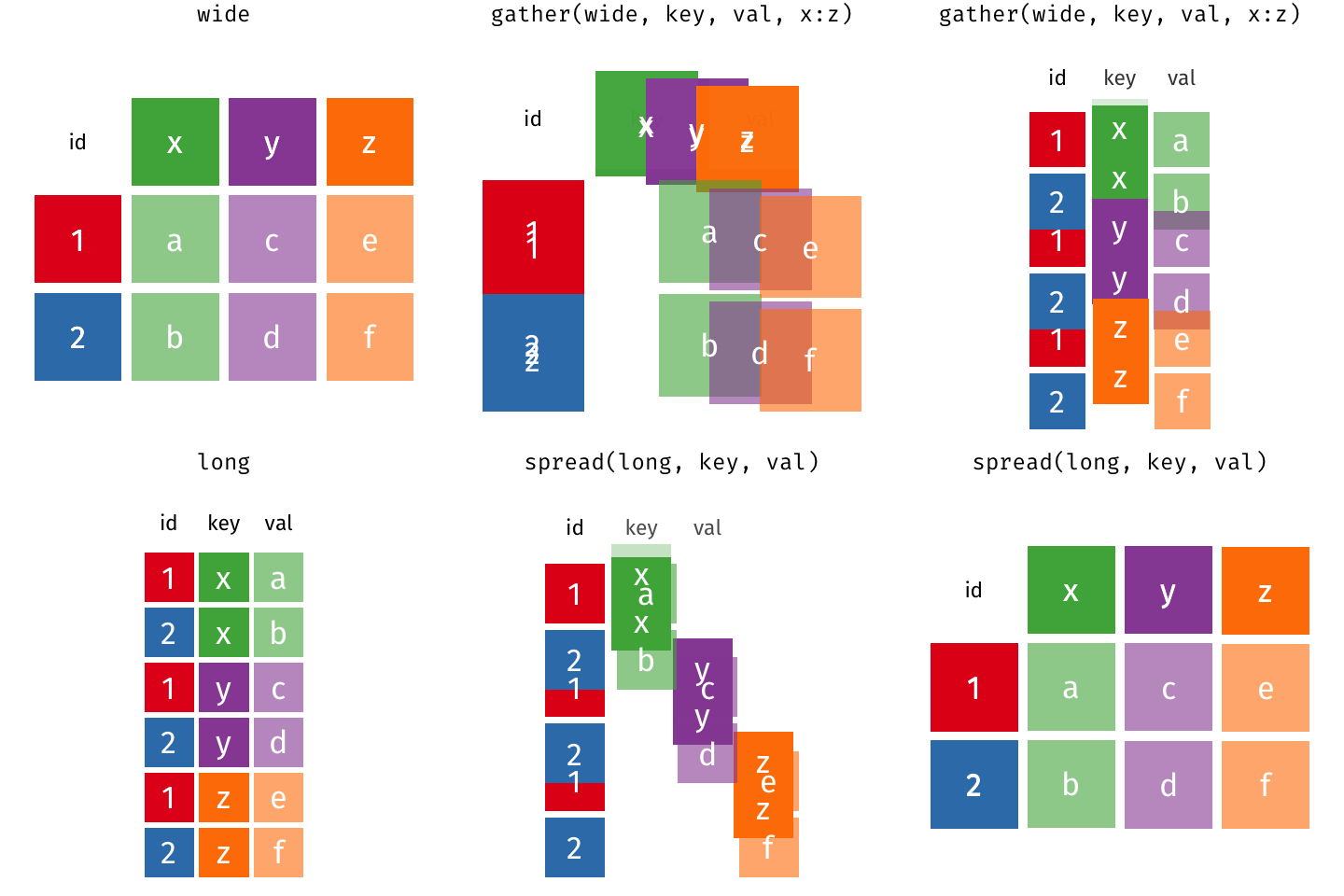
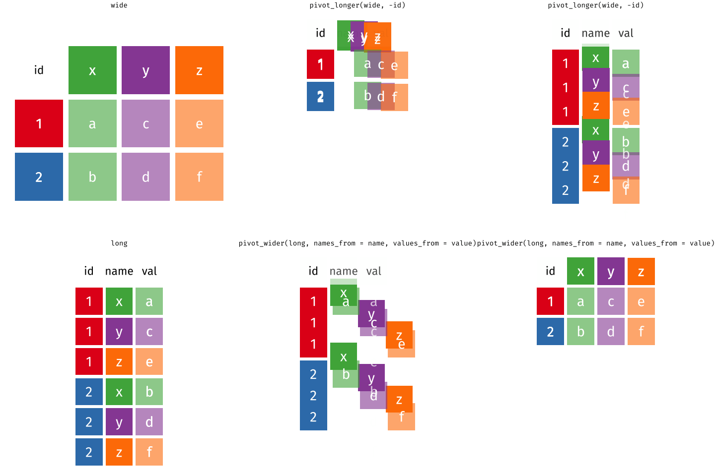
We will often need to reshape our datasets and should have a way to go:
- from wide format to long (tidy) format using
gatherorpivot_longer - from long (tidy) to wide format using
spreadorpivot_wider
In a set of wonderful animations from Garrick Aden-Buie, this is the process of coverting from long format to wide and back


Let us review the basic tasks for tidying data using the R for Data Science gapminder subset.
## # A tibble: 6 x 4
##   country      year  cases population
##   <chr>       <int>  <int>      <int>
## 1 Afghanistan  1999    745   19987071
## 2 Afghanistan  2000   2666   20595360
## 3 Brazil       1999  37737  172006362
## 4 Brazil       2000  80488  174504898
## 5 China        1999 212258 1272915272
## 6 China        2000 213766 1280428583
Note that in this data frame, each variable is in its own column (country, year, cases, and population), each observation is in its own row (i.e. each row is a different country-year pairing), and each value has its own cell.
9.1.1 pivot_longer or gather data
Gathering entails bringing a variable spread across multiple columns into a single column. For example, this version of table1 is not tidy because the year variable is in wide format, spread across multiple columns:
## # A tibble: 3 x 3
##   country     `1999` `2000`
## * <chr>        <int>  <int>
## 1 Afghanistan    745   2666
## 2 Brazil       37737  80488
## 3 China       212258 213766
The variables (columns) that a tidy dataframe would have would be country, year, and cases. We can use the pivot_longer or gather() function from the tidyr package to reshape the data frame and make this tidy. To do this we need three pieces of information:
- The names of the columns that represent the values, not variables. Here, those are
1999and2000. - The
key, or the name of the variable whose values form the column names. Here that isyear. - The
value, or the name of the variable whose values are spread over the cells. Here that iscases.
Notice that we create the names for
keyandvalue- they do not already exist in the data frame.
We implement this using the pivot_longer() or gather() function. pivot_longer() requires the newest version of tidyr from github, so you need to reinstall tidyr as shown below:
Once you have installed the newest version of tidyr, then you can use either pivot_longer() or gather()
## # A tibble: 6 x 3
##   country     year   cases
##   <chr>       <chr>  <int>
## 1 Afghanistan 1999     745
## 2 Afghanistan 2000    2666
## 3 Brazil      1999   37737
## 4 Brazil      2000   80488
## 5 China       1999  212258
## 6 China 2000 213766## # A tibble: 6 x 3
## country year cases
## <chr> <chr> <int>
## 1 Afghanistan 1999 745
## 2 Brazil 1999 37737
## 3 China 1999 212258
## 4 Afghanistan 2000 2666
## 5 Brazil 2000 80488
## 6 China 2000 213766This operation would be called reshaping data wide to long.
9.1.2 pivot_wider or spread data
If we wanted to make a long table into a wide one, we use pivot_wider; spreading brings an observation spread across multiple rows into a single row. It is the reverse of gathering, or taking a wide dataset and making it long. For instance, take table2:
## # A tibble: 12 x 4
##    country      year type            count
##    <chr>       <int> <chr>           <int>
##  1 Afghanistan  1999 cases             745
##  2 Afghanistan  1999 population   19987071
##  3 Afghanistan  2000 cases            2666
##  4 Afghanistan  2000 population   20595360
##  5 Brazil       1999 cases           37737
##  6 Brazil       1999 population  172006362
##  7 Brazil       2000 cases           80488
##  8 Brazil       2000 population  174504898
##  9 China        1999 cases          212258
## 10 China        1999 population 1272915272
## 11 China        2000 cases          213766
## 12 China        2000 population 1280428583
It violates the tidy data principle because each observation (unit of analysis is a country-year pairing) is split across multiple rows. To tidy the data frame, we need to know:
- The
keycolumn, or the column that contains variable names. Here, it istype. - The
valuecolumn, or the column that contains values for multiple variables. Here it iscount.
Notice that unlike for gathering, when spreading the
keyandvaluecolumns are already defined in the data frame. We do not create the names ourselves, only identify them in the existing data frame.
## # A tibble: 6 x 4
##   country      year  cases population
##   <chr>       <int>  <int>      <int>
## 1 Afghanistan  1999    745   19987071
## 2 Afghanistan  2000   2666   20595360
## 3 Brazil       1999  37737  172006362
## 4 Brazil       2000  80488  174504898
## 5 China        1999 212258 1272915272
## 6 China 2000 213766 1280428583## # A tibble: 6 x 4
## country year cases population
## <chr> <int> <int> <int>
## 1 Afghanistan 1999 745 19987071
## 2 Afghanistan 2000 2666 20595360
## 3 Brazil 1999 37737 172006362
## 4 Brazil 2000 80488 174504898
## 5 China 1999 212258 1272915272
## 6 China 2000 213766 1280428583This operation would be called reshaping data long to wide.
9.1.3 Separating
Separating splits multiple variables stored in a single column into multiple columns. For example in table3, the rate column contains both cases and population:
## # A tibble: 6 x 3
##   country      year rate
## * <chr>       <int> <chr>
## 1 Afghanistan  1999 745/19987071
## 2 Afghanistan  2000 2666/20595360
## 3 Brazil       1999 37737/172006362
## 4 Brazil       2000 80488/174504898
## 5 China        1999 212258/1272915272
## 6 China        2000 213766/1280428583
This is a bad idea as you lose information. Tidy data principles require each column to contain a single variable. We can use separate() to split the column into two new columns:
## # A tibble: 6 x 4
##   country      year cases  population
##   <chr>       <int> <chr>  <chr>
## 1 Afghanistan  1999 745    19987071
## 2 Afghanistan  2000 2666   20595360
## 3 Brazil       1999 37737  172006362
## 4 Brazil       2000 80488  174504898
## 5 China        1999 212258 1272915272
## 6 China        2000 213766 1280428583
9.1.4 Uniting
Uniting is the inverse of separating - when a variable is stored in multiple columns, uniting brings the variable back into a single column. table5 splits the year variable into two columns:
## # A tibble: 6 x 4
##   country     century year  rate
## * <chr>       <chr>   <chr> <chr>
## 1 Afghanistan 19      99    745/19987071
## 2 Afghanistan 20      00    2666/20595360
## 3 Brazil      19      99    37737/172006362
## 4 Brazil      20      00    80488/174504898
## 5 China       19      99    212258/1272915272
## 6 China       20      00    213766/1280428583
To bring them back, use the unite() function:
## # A tibble: 6 x 3
##   country     new   rate
##   <chr>       <chr> <chr>
## 1 Afghanistan 19_99 745/19987071
## 2 Afghanistan 20_00 2666/20595360
## 3 Brazil      19_99 37737/172006362
## 4 Brazil      20_00 80488/174504898
## 5 China       19_99 212258/1272915272
## 6 China 20_00 213766/1280428583## # A tibble: 6 x 3
## country new rate
## <chr> <chr> <chr>
## 1 Afghanistan 1999 745/19987071
## 2 Afghanistan 2000 2666/20595360
## 3 Brazil 1999 37737/172006362
## 4 Brazil 2000 80488/174504898
## 5 China 1999 212258/1272915272
## 6 China 2000 213766/1280428583If we wanted to make gapminder a tabular, wide dataframe, we would use pivot_wider()
gapminder_life_exp_wide  <- gapminder %>%
  select(country, continent,
         lifeExp, year) %>%
  pivot_wider(names_from = year, values_from = lifeExp)


  gapminder_life_exp_wide
## # A tibble: 142 x 14
## country continent `1952` `1957` `1962` `1967` `1972` `1977` `1982` `1987`
## <fct> <fct> <dbl> <dbl> <dbl> <dbl> <dbl> <dbl> <dbl> <dbl>
## 1 Afghan~ Asia 28.8 30.3 32.0 34.0 36.1 38.4 39.9 40.8
## 2 Albania Europe 55.2 59.3 64.8 66.2 67.7 68.9 70.4 72
## 3 Algeria Africa 43.1 45.7 48.3 51.4 54.5 58.0 61.4 65.8
## 4 Angola Africa 30.0 32.0 34 36.0 37.9 39.5 39.9 39.9
## 5 Argent~ Americas 62.5 64.4 65.1 65.6 67.1 68.5 69.9 70.8
## 6 Austra~ Oceania 69.1 70.3 70.9 71.1 71.9 73.5 74.7 76.3
## 7 Austria Europe 66.8 67.5 69.5 70.1 70.6 72.2 73.2 74.9
## 8 Bahrain Asia 50.9 53.8 56.9 59.9 63.3 65.6 69.1 70.8
## 9 Bangla~ Asia 37.5 39.3 41.2 43.5 45.3 46.9 50.0 52.8
## 10 Belgium Europe 68 69.2 70.2 70.9 71.4 72.8 73.9 75.4
## # ... with 132 more rows, and 4 more variables: `1992` <dbl>, `1997` <dbl>,
## # `2002` <dbl>, `2007` <dbl>Similarly, if we wanted to convert from the wide gapminder to the long one, we would use either gather or pivot_longer()
gapminder_life_exp_wide %>%
  gather(key = "year", value = "lifeExp",
         -country, -continent) %>%
  mutate(year = as.numeric(year))
## # A tibble: 1,704 x 4
## country continent year lifeExp
## <fct> <fct> <dbl> <dbl>
## 1 Afghanistan Asia 1952 28.8
## 2 Albania Europe 1952 55.2
## 3 Algeria Africa 1952 43.1
## 4 Angola Africa 1952 30.0
## 5 Argentina Americas 1952 62.5
## 6 Australia Oceania 1952 69.1
## 7 Austria Europe 1952 66.8
## 8 Bahrain Asia 1952 50.9
## 9 Bangladesh Asia 1952 37.5
## 10 Belgium Europe 1952 68
## # ... with 1,694 more rowsgapminder_life_exp_wide %>%
pivot_longer(
cols = c(-country, -continent), #keep country and continent
names_to = "year",
values_to = "lifeExp",
) %>%
mutate(year = as.numeric(year)) ## # A tibble: 1,704 x 4
## country continent year lifeExp
## <fct> <fct> <dbl> <dbl>
## 1 Afghanistan Asia 1952 28.8
## 2 Afghanistan Asia 1957 30.3
## 3 Afghanistan Asia 1962 32.0
## 4 Afghanistan Asia 1967 34.0
## 5 Afghanistan Asia 1972 36.1
## 6 Afghanistan Asia 1977 38.4
## 7 Afghanistan Asia 1982 39.9
## 8 Afghanistan Asia 1987 40.8
## 9 Afghanistan Asia 1992 41.7
## 10 Afghanistan Asia 1997 41.8
## # ... with 1,694 more rows9.2 RStudio primer on tidyr
Recent versions of tidyr have renamed these core functions:
gather()is nowpivot_longer()andspread()is nowpivot_wider(). The syntax for thesepivot_*()functions is slightly different from what it was ingather()andspread(), so you can’t just replace the names. Even though, bothgather()andspread()still work and won’t go away for a while, I think tt’s worth learning the newerpivot_*()functions.
9.3 More resources
- Pivoting data from columns to rows (and back!) in the tidyverse
- Pivoting in
tidyr - Hadley Wickham’s tidy data paper
This page last updated on: 2020-07-15